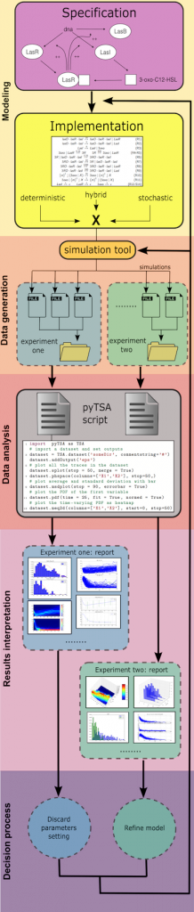
Analysis of dynamical systems is often done via simulation ensembles, under different parameter configurations, or by repeatedly sampling from a random process. In any case, automatizing time-series analysis is key to save time and focus on other tasks, e.g. model refinement.
pyTSA is a Python tool to make time-series analysis as intuitive as possible. Its scripts can be pipelined with any simulation tool outputting time-series, and intuitive commands allow to perform complex analyses in a intuitive way.
Reference: Antoniotti, M., De Sano, L., Garavagna, G. (2014). pyTSA: Analysis of stochastic biochemical time-series made easy. 11th Annual Meeting of the Bioinformatics Italian Society (BITS 2014).
Input and output data
A dataset is a set of files in the usual csv/tsv/.. format; each file is interpreted as the result of an experiment, e.g. a model simulation, where each column is a variable of your system. pyTSA can load whole datasets (or portions) in a multi-threading fashion by using the very simple command dataset, or specific time-series by using command timeseries.
Whenever data is loaded a pyTSA object is available to perform plots, which can be exported in png/eps/raw/.. formats. To make scripting more readable, columns can be assigned names to reference afterwards.
then load a dataset in folder Dir and name the columns t (time), Preys and Predators. Any pyTSA function can be called on called on the returned object obj.
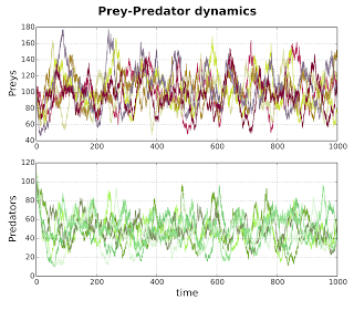
You can plot as many time-series as you want from a loaded dataset, possibly separating each system variable (i.e., columns) in separate panels, as shown in this panel. This is especially useful when variables spans over different magnitudes.
Also, one can plot 2D/3D phase spaces to understand the relation between two/three system variables by calling the phspace function.
Example: Simple plot (splot) on separate panels (merge=False) of the columns named Preys and Predators, for time below 1000. This plots all the traces in the loaded dataset object obj
What is the "average" behavior emerging from my data?
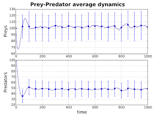
To ensemble different experiments and gain a “average” behavior one can easily compute the average of all the time-series.
This information is useful for instance to predict the expected value of a system variable when the model which generated data is a stochastic process.
As usual, together with the expected value one can plot the standard deviation of a variable. This is the simplest of all the aggregate measure implemented in pyTSA.
Example: Plot of averages and standard deviation (asdplot) on separate panels of the columns for Preys and Predators, with 20 error bars.
obj.asplot(..., errorbar=True, numbars=20)
What is the probability of finding X units of chemical Y after Z time units?
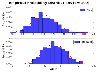
Imagine that your model describes the interactions of some chemical Y. If you performed many different experiments with your model, you might want to evaluate the probability of chemical Y to be present in X units, after Z time units from the initial simulation time.
This probability density function can be evaluated with the native pyTSA command pdf, in a very simple fashion. Also, the distribution can be normalized and fit with a Gaussian, if required, and multiple time-points can be used at once.
Example: At time 100 plot and fit the normalized distributions (pdf) of the columns Preys and Predators.
obj.pdf(100, ..., merge=False, fit=True)
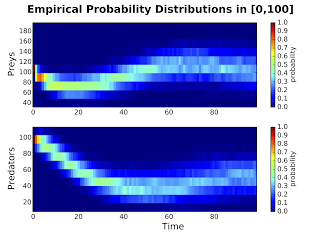
What is the probability of finding X units of chemical Y at any time point?
One might be interested in estimating the probability of observing certain units X of chemical Y all along the model execution.
From the point of view of stochastic models, this is equivalent to assess, for the chemical Y, the solution of its master equation which rules the change, in time, of such a probability. Since for most models this equation is not solvable, its solution is often estimated by numerical ensembles, as in pyTSA.
Command meq allows to easily estimate this quantity, and plots it either as a heatmap or a 3D surface.
Example: For time in [0,100] estimate the time-varying probability of the columns Preys and Predators and visualize it as a heatmap (meq2d)